Stribeck Friction Calculator for Elliptical Contact: Online

TriboNet

30.09.2021

Friction in Mixed Lubrication Regime

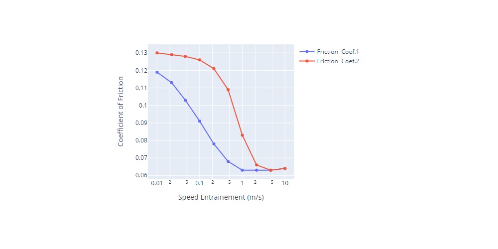
This online calculator allows qualitative estimation of the friction coefficient in a mixed lubricated elliptical (point) contact. The theory behind this tool is given below the calculator.

Calculating Stribeck Curve

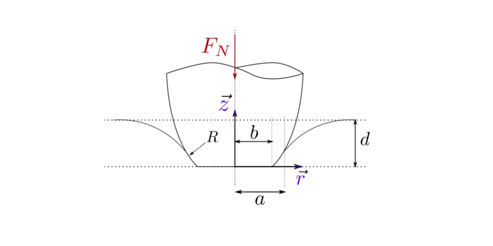
This calculator is based on the load-sharing concept that can be used to calculate friction in mixed lubrication regime approximately, but very fast and in a robust way. The concept, first introduced by Johnson [1], offers advantages of robustness, significantly reduced computational requirements and a relative simplicity. In these models the general problem is split up into two problems: lubrication problem assuming smooth surfaces and a “dry” rough contact problem, for details see [2]. In this case the flow equations are solved assuming that the surfaces in contact are smooth, while the “dry” contact problem assumes that there is no lubricant between the surfaces. These problems are linked via the load carried by the lubricant and by the “dry” contact [3], see figure below.

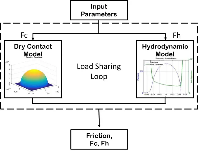
Load sharing friction model — Load sharing concept for friction calculation [3].

In the simplest form, the load-sharing concept can use a central film thickness fit to calculate the lubricant film thickness for the lubrication problem and Greenwood-Williamson model (GW) for the “dry” contact problem. This approach can give a good qualitative prediction of the friction evolution, however, it is likely to overestimate friction due to assumptions used in both GW model (assumption of the independent asperity deformation, which overestimates the load carried by asperities) and central film thickness calculations (assumption of a constant film thickness in the contact area, which is true only for “highly” loaded cases), see [3]. Current calculator uses this approach.

Determination of Roughness Parameters

The GW model and this calculator uses 3 parameters to describe the rough surface: density of asperities $n$ , mean radius of asperities $\beta$ and standard deviation of asperities height $\sigma$ . These parameters can be calculated as discussed below.

The density of asperities requires the definition of what asperity is. Here, asperity is defined as a point on the surface which is higher than its 8 neighbors, as shown in the figure below.

asperity definition — Definition of asperity

By counting the number of such asperities for a given surface and dividing it by the surface area, one can obtain the density of the asperities per unit area.

The mean readius of asperities can be calculated as follows:

(1) $\begin{eqnarray*} \beta_x^{-1} = \frac{z_{x-\Delta x,y} - 2z_{x,y} + z_{x+\Delta x,y}}{\Delta x^2} \\ \beta_y^{-1} = \frac{z_{x,y-\Delta y} - 2z_{x,y} + z_{x,y+\Delta y}}{\Delta y^2} \end{eqnarray*}$

where $\beta_x, \beta_y$ are the radii of curvature in $x,y$ directions respectively, $z_{x,y}$ is the height at location $(x,y)$ and $\Delta x,\Delta y$ are the roughness measurement resolution (pixel size). The asperity radius $\beta$ is then calculated as follows:

(2) $\begin{eqnarray*} \beta = \sqrt{\beta_x \beta_y} \end{eqnarray*}$

By calculating the radius for each asperity on the surface and taking the average, one can obtain the mean asperity diameter that is used in the calculator above. In case of the contact of two surfaces the mean radius of asperities is calculated as follows:

(3) $\begin{eqnarray*} \frac{1}{\beta} = \frac{1}{\beta_1} + \frac{1}{\beta_2} \end{eqnarray*}$

where $\beta_1$ and $\beta_2$ are the mean radii of asperities for surface 1 and 2 correspondingly. The standard deviation of the asperities heights is calculated as follows:

(4) $\begin{eqnarray*} \sigma_s^2 = \frac{1}{n} \sum_{i=1}^{n} (h_i - d_d)^2 \end{eqnarray*}$

where $h_i$ is the height of the $i$ -th asperity, $d_d$ is the distance between the mean height of the asperities and the mean height of the whole surface. For two surfaces, the standard deviation of the asperity heights is calculated as follows:

(5) $\begin{eqnarray*} \sigma_s = \sqrt{\sigma_s_1^2 + \sigma_s_2^2} \end{eqnarray*}$

Here $\sigma_s_1^2$ and $\sigma_s_2^2$ are the standard deviation of the asperity heights for surface 1 and 2 correspondingly.

Further details on this approach can be found in the PhD Thesis by Irinel Faraon, 2005, University of Twente.

References:

[1] Johnson KL, Greenwood JA, Poon SY. A Simple Theory of Asperity Contact in Elasto-Hydrodynamic Lubrication. Wear. 1972;19:91-108.

[2] Zhu D, Hu Y-Z. A computer program package for the prediction of EHL and mixed lubrication characteristics, friction, subsurface stresses and flash temperatures based on measured 3-D surface roughness. Tribology Transactions. 2008;44:383-90.

[3] Akchurin, A., Bosman, R., Lugt, P.M. et al. On a Model for the Prediction of the Friction Coefficient in Mixed Lubrication Based on a Load-Sharing Concept with Measured Surface Roughness. Tribol Lett 59, 19 (2015). https://doi.org/10.1007/s11249-015-0536-z

[4] Irinel Faraon, PhD Thesis, 2005, University of Twente