Elastohydrodynamic Lubrication (EHL): Theory and Definition

What is Elastohydrodynamic Lubrication (EHL)?

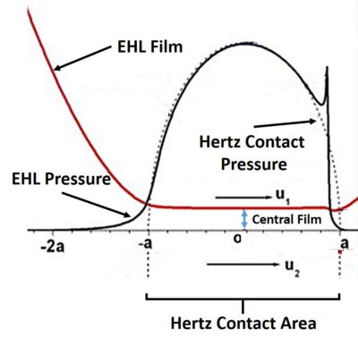
Elastohydrodynamic Lubrication – or EHL – is a lubrication regime (a type of hydrodynamic lubrication (HL)) in which significant elastic deformation of the surfaces takes place and it considerably alters the shape and thickness of the lubricant film in the contact. The term underlies the importance of the elastic deflection of the bodies in contact in the development of the total lubricant film. EHL, the same way as HL, is used to decrease friction and wear in tribological contacts. It is achieved by the development of a thin lubricant film between rubbing surfaces, which separates them and decreases friction. EHL has characteristic features, such as constant film thickness and almost Hertzian contact pressure profile within the Hertzian contact area, as shown in the figure below. These features have been extensively used in construction of approximate solutions of EHL theory.

History of EHL

Classical Hydrodynamic Lubrication (HL) theory assumes the bodies to be rigid. In 1916 Martin obtained a closed form solution of the Reynolds equation for a film thickness and pressure in a cylinder and plane geometry assuming rigid surfaces and isoviscous lubricant. But comparison with experimental data revealed significant discrepancy with the model predictions. Divergence of experimental and theoretical results leaded researchers to the conclusion that elastic distortion and pressure-viscosity effect play a significant role in lubrication. In 1949, Grubin obtained a first solution (approximate) for elasto-hydrodynamic lubrication problem assuming a cylinder on flat geometry. He was the first to include both elastic deformation and piezoviscous behavior of the lubricant into theoretical solution. Although his solution is only approximate, his analysis is quite accurate under certain conditions and it was recognized as a big step forward in EHL theory (since then the term EHL has been used). Moreover, Grubin’s assumptions are widely used in the modern tribology to build various approximate solutions under highly loaded contacts [1]. The derivation, Matlab code and detailed analysis of Grubin solution is considered here.

Petrushevich (Petrusevich 1951) was actually first to obtain the exact solution of the line contact EHL problem by solving the corresponding equations numerically. He was also the first to observe a pressure spike at the outlet of the contact – a characteristic feature of EHL (see the figure above). For this reason the feature is sometimes referred to as “Petrushevich” spike. Obtained in 1951, his solution was first solution of combined elastic distortion, fluid flow and pressure-viscosity dependency equations. It should be emphasized, that the occurrence of the pressure spike is closely related to the variance of viscosity with pressure along with elastic properties of materials and relative speed. In 1959 Dowson and Higginson computed series of numerical solutions of EHL line contact problem for a range and obtained a regression formula for a minimum film thickness. Further information on the development of the EHL theory can be found in [2].

System of EHL equations

A classical EHL system of equations consists of the system of Reynolds equation, film thickness and load balance equations:

(1)  

where are hydrodynamic film thickness, pressure, viscosity, and and represent the velocity of the bearing surfaces. Variables represent the approach, macroscale geometry, elastic distortion of the surfaces and microscale geometry (surface roughness) correspondingly. This system of equations can be solved assuming appropriate boundary conditions to obtain unknown hydrodynamic pressure and film thickness in the contact. Typically, parameter is unknown (although sometimes it can be specified), therefore the last integral equation is needed to get the closed system of equations. is the normal load applied to the contact.

The system of equations  shown above can be solved analytically in certain cases, however, in general it has to be solved using numerical methods. The problem in solving the Reynolds equation comes from the film thickness equation, when the elastic deflection of the surfaces is not negligible. For a 2-D case, this term can be calculated from the following equation:

(2)  

where is the reduced elastic modulus. This equation is the analytical solution of the theory of elasticity equations for a semi-infinite body subjected to normal pressure (for the details of the derivation refer to [3]). The most robust and fast way (in terms of iterations at least) to solve EHL system is to use a fully coupled approach and Newton’s scheme. However, since the elastic distortion equation is given in the integral form, the Jacobian of the system is full which increases the demands in memory enormously. In addition, solution of the equations with full Jacobian is computationally significantly more intense compared to diagonally banded cases.Therefore, researchers worked hard to develop alternative solution methods. The two most common methods for solving EHL systems numerically are the Multilevel-Multigrid and Differential Deflection techniques. The former uses multiple grids and specific integration of the film thickness equation to build an iterative solver [5]. The latter solves a fully coupled system of equations, however, instead of using the original integral form of the film thickness equation, it considered the 2-nd derivative of it [4,6]. It turns out that the use of the derivative equation allows to construct a banded Jacobian and improve the efficiency of coupled approach significantly.

Recently, a so called full system approach was proposed [7]. In this case, a Finite Element Methods are used to calculate both Reynolds and elasticity equations in a coupled manner. This method is computationally more demanding since the subsurface volume has to be discretized to calculate elastic distortions (the fully coupled approach based on differential deflection is faster than the FEM based full system technique). Nevertheless, the approach has the advantage of flexibility since it can be developed using commercial software such as COMSOL.

A Matlab code for the solution of EHL system for the case of a cylinder-on-disk can be found here or for the cases of high pressures here. A fully coupled approach based on differential deflection technique was utilized. Newtons scheme was employed.

Film Thickness Measurements

Since the film thickness controls the separation of the rubbing surfaces and consequently friction, researchers developed several ways to measure the hydrodynamic film in the contact. One of the most frequently used techniques is based on optical interferometry. The instrument measures the lubricant film thickness in the contact formed between a steel ball and a rotating glass disc covered by a specific layer. The lubricant film thickness at any point in the image can be accurately calculated by measuring the wavelength of light at that point. Film thicknesses down to 1 nm can be measured by this approach. You can see the measurement of the film in the video below (at first the disk is stationary and later on stats the motion):

Central and minimum film thickness: Online EHL film thickness calculator

As it can be clearly seen from the Fig.1, the lubricant film thickness is more or less constant in the whole contact zone (where the pressure is large), except for the small area at the outlet, where the film thickness drops to its minimum value. Since the pressurized area is typically the most important for failure analysis, in practice engineers use only central film thickness and the minimum film thickness to describe the lubrication state (see this article for more details).
An online film thickness calculator is available on tribonet for line and elliptical (point) contacts. The calculators allow calculating central and minimum film thicknesses using various equations. Exact equations are described on the calculator’s page. Here is the calculator for elliptical contact: