Administration of the project
Contact Pressure For Rough Surfaces: A Tutorial
08.11.2017
Update 13-02-2022: Currently, a cloud based tool for the calculation described below is available. Please refer to the example given here.
In this article, a calculation of contact pressure in a rough contact is discussed. The calculation is done using a Tribology Simulator software, which is available for download here (its free to use). The simulator uses a Boundary Element Method (BEM) with Fast Fourier Transform and Conjugate Gradient method to obtain the contact pressure and the real contact area at a contact of two rough surfaces (it can also be used to calculate subsurface stresses and other kind of tribology related problems). The model is based on the half-space theory approximation. In a recently published Contact Mechanics Challenge results, it was shown that BEM based approach (along with a computationally demanding Green’s Functions approach) is the most accurate way to calculate contact pressure for rough surfaces.
Half-Space Approximation
As of today, the most efficient way in terms of the accuracy and efficiency, BEM based approach is the most suitable way of characterizing contact situation between rough surfaces (this also includes subsurface stress calculation, stiffness and pre-sliding analysis). This is due to the fact that other methods, such as Finite Element Methods, or Molecular Dynamic models are much more computationally intense and solution of many practical problems is not feasible. BEM solution is based on the solution of the classical equations of the theory of elasticity for a semi-infinite half-space with homogeneous mechanical properties (although BEM approach was also extended for layered surfaces, and non-homogeneous surfaces as well). For such a half-space, the elastic deflection is given in a form of an integral (as discussed in more detailed manner here):
(1) 

Here  is the elastic deflection,
  is the reduced elastic modulus,
  are the Poisson’s ratio and Young’s modulus of the bodies,
  is the contact pressure. This equation is used in most of tribological problems involving rough surfaces, including EHL problems, but also in contact analysis, friction and wear simulation.
The system of equations to be solved in this case looks as follows:
(2) 
Here,  is the combined surface roughness of the surfaces,
  is the rigid body approach and
  are the contact area and applied normal load correspondingly. Once the system is solved, one gets the contact pressure and the real contact area. This system of equations can be extended to consider the plastic behavior of the materials as well as to have friction on the surface and coatings.
Tribology Simulator
Tribology Simulator is a stand-alone software for tribological analysis. First, it should be downloaded and launched (you will also need to download an MCR installer from MATLAB site, see the readme file). A following window will show up:

On the left side, the global settings steps of the problem are shown. You start with the selection of the Simulation Type, which in the current article is the dry contact simulation. Next, the macroscopic geometry is set. This can be a cylindrical, spherical, elliptical shape or just a flat. It is instructive to use a sphere here as an example. The radius of the sphere is chosen in the table. It should be noted that the settings for the simulation can be loaded from the file (previously saved). For simplicity, it is good to do so: on the context menu, click File, Load parameters. In the dialogue window, go to the Examples\Contact Pressure Calculation and select ‘Parameters.mat’ file. All the simulation settings will be imported.
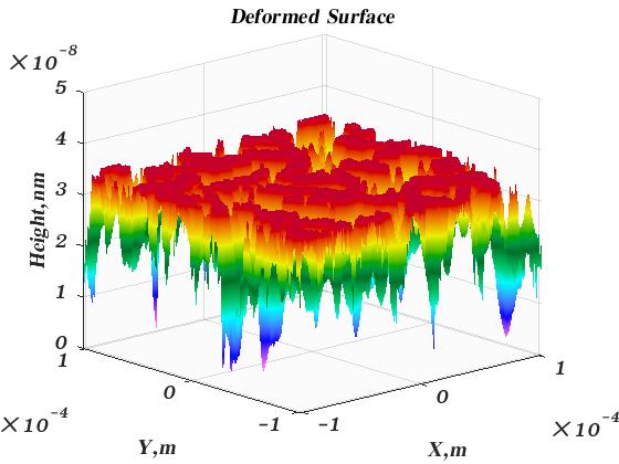
At the next step, it is necessary to define the microscopic geometry, which is known in tribology field as roughness (there is a possibility to consider a smooth contact analysis as well, then the solution will be identical to the Hertz contact solution). In this post, we will consider an artificially generated surface (you can do it by choosing Tools/Surface Generator), which is located at the same place as the parameters file imported on the previous step. Although it is not necessary, it is instructive to take a look how does the surface roughness look. For that, click the Import Roughness button and choose the Examples\Contact Pressure\Surface Roughness.csv file (it is also possible to import surfaces in other formats) and if everything is alright, you will see the profile on the graphic panel. Some parameters of the surface will also be shown to the left from the plot. It should be noted, that the original surface is interpolated to the numerical grid which is defined later on. This particular file is just a matrix of of heights in meters. It is important in this case to manually define the resolution of the roughness profile in the corresponding table.
Now go further to the Contact Model. There are several available, but for now we use Half-Space Based model (see the Help\Manual for the description of other models). It is also possible to calculate the subsurface stress (check this option if you would like to do that as well, but be careful it gets more time consuming).
With the next step, you can specify the properties of the bodies in contact. In the corresponding table you specify Elastic modulus in Pa, Poisson’s ratio (dimensionless) and the hardnesses of the materials (in Pa). If you want to perform purely elastic calculations, set the hardness values to a very high value. The half-space approximation theory was also used to get the solution for the coated surfaces (layered). In Tribology Simulator, there is also an option to consider a single layer on top of each of the surfaces (see more details in the manual).
In the next step, it is necessary to choose the friction model. The friction of the surface impacts the contact pressure, since the shear forces introduces displacements and this is taken into account in the model. The simplest model is the Coulomb model and it is assumed then that the coefficient of friction (COF) is constant. For the current simulation, 0 COF can be chosen simulating traction free surface.
Now go to contact conditions (we skip the wear, thermal and tribochemical models in this article) to choose the contact (normal) load. In this table, for dry contact pressure analysis only the load has to be set (you can also specify several loads using a whitespace as a separator). Here you also need to specify the boundary conditions. In the current simulation, no periodic boundary condition is used (so 0 pressure at the outside). In the table at the bottom of the panel, the hertz parameters are calculated. These parameters can be used to set the dimensions of the computational grid. For example, if the Hertz contact radius is 200  , then the computational domain should be at least twice as this value.
The last step in this simulation set up is the setting of the numerical grid. That is on the Contact Grid panel. In the table, in the first row you need to enter the length of the numerical grid in x and y directions (also in z direction, if you calculate subsurface stresses). In the second row you need to specify the number of grid points. The last row will show the resolution of the grid (it will be calculated as the length divided by the corresponding number of grid points).
Now you can proudly press the big bang Run button. The simulator will ask you to choose the roughness file. You will see a small progress text on the left bottom part of the simulator window. If you consider more than one load, it will show you the progress of the simulation. In the Windows Command Shell window, you will be updated as well. You can now choose the Results row and once the simulation is over, the new window will appear and the last calculated results will be loaded.
On the Results panel, it is possible to plot the calculated variables. In our case, we are interested in the contact pressure. So we choose Contact Pressure in the listbox and click plot. A pressure profile like this will be shown:
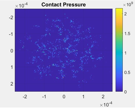
This is how the pressure profile at the contact interface look like (the scale is in Pa unit). It is possible to export this data by clicking Export button (you can export it to matlab or csv file). It is obvious here, that the Hertz radius approximately encircles the contact area here as well (the Hertzian radius is found in the table at the Contact Conditions panel).
I hope this helps!
Leave a Reply
You must be logged in to post a comment.
HELLO SIR
MANY THANKS FOR YOUR ARTICLE HOW FRICTION SURFACE CAN BE CALCULATED WITH MATHEMATICAL MODEL , I AM SPIRAL PAPER TUBE CORE MAKER I AM FACING CRITICAL PROBLEM OF FRICTION CRATED BETWEEN METAL ROUND CYLINDER&PAPER WHILE FORMING PAPER CORE NAY SUITABLE WAX CAN REDUCE FRICTION IN MY PROBLEM IF SO LET ME KNOW IN THIS MATTER
You can use the model described in the post to calculate the contact area. Given that, you can multiply the contact area by the effective shear strength. This gives you the friction force. Unfortunately, the effective shear strength can be obtained only from the experiments.
Dear Sir
You’ve done a very good job. Can you send the codes in the Tribology Simulator for the calculation of Elastic deformation, contact pressure, subsurface stress, and so on.Best wishes.
hello,I installed the matlab R2014a. In order to execuate the Tribology Simulator, I installed Matlab runtime 9.2 as well, but the execuative file connot open, why?
Hello! Does the black screen appear at all? If so, you can take a look what is the error message. Also keep in mind, that when you open it for the first time, it may take a while. If you put it into network directory, it may be difficult to open the executable. So place it on the local drives and see if it works. Please let me know, if it worked out.
Hello,
I am using this free program for my masters dissertation. I am interested in obtaining contact pressure fields for dry rough contacts. I managed to obtain promising results with the half-space based model, but unfortunately now, with the same input parameters, the simulation results look Hertzian! It looks like there is a bug or something prevents the software from using the csv file (even though it resolved it fine before). Can you please help me understand what the issue is and how it can be resolved? Thank you!
Hi, Thank you for the amazing software.
Is it possible to use it programmatically (on a Matlab script) in order to loop on different micro-geometries? I am having trouble launching the Tribology simulator from a script.
Thank you very much.
Hi! Yes, you can do that. For that you need to pass the Input.mat file as follows from Matlab: system(‘tribology_simulator.exe Inputs.mat’); The file Inputs.mat is the matlab file with the structure that contains all the necessary input, including the file used in the contact calculations. To update the micro-geometries, you need to first load the Inputs.mat into Matlab, then change the roughness file name in the Input structure as follows: Input.FileName1 = FullPathToFile; Here FullPathToFile is the path to the surface file. Then you need to save the file into Inputs.mat. In this way you can make a loop over the surfaces.
Amazing, Thank you very much, I will test this and get back to you!
Hi, Thank you for your answer.
I managed to run the Tribonet software in a loop by passing the new Input.mat file which I modified and it seems to work.
Nevertheless, I cannot manage to recover the data from the ‘SAVE’ folder. It seems that it is not updating the ‘current_data’ structures properly since all the results from my loop are the exact same (for very different rough surfaces). I am recovering the results in the loop each time from the ‘ContactOutputGlobal’ cell.
Do you know if there is any reason why the current_data structure is not getting updated from the programatic call to the executable (I wonder if this is the reason why I get always the same results)?
Thank you very much.
Best regards
Hi!
I think it updates the current_data at every loop, so you need to save the current_data file every iteration. Please check this option and let me know it this works
Hi, sorry for the delay in my answer! This works thank you very much!
Best regards,
Mateo Acosta
Hi. Quick Yes / No Question! Do I need MatLab to run the Tribology Simulator?
Many thanks.
Hi Kevin!
Actually, you dont need Matlab, you only need matlab runtime. That one you can download for free on Matlab website. Alternatively, you now can use an online version of the simulator: https://tribology.eu/.
I tried using online simulator. But in Micro Geometry, it is asking to import files.
What do I need to import actually?
Can you please share that file?
Thank you.