Flash Temperature Calculator

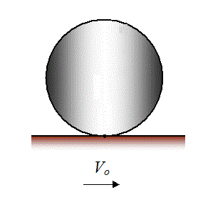
In tribological contacts, regardless of their lubrication regime, heat generated by friction affects the properties of the system. Lubricant viscosity can change, surfaces can oxidize, and melting can even change the contact geometry. The tribological performance of the whole system may also be altered. For example, once a certain temperature is exceeded, mild wear may change abruptly to a more severe wear mode, with increased wear and friction.

Several theories have been proposed to describe this transition or failure criterion, including friction-power criteria (Meng, 1960) and friction-power-intensity criteria (Matveevsky, 1965). Most are related to heat generated in the contact. An influential temperature-based theory was formulated by Blok (1939) and later developed by Bos (1995), van Drogen (2005), and Bosman (2011).

In mixed and boundary lubrication, heat has two principal sources: shearing of the liquid layers and friction in surface-asperity contacts. Because asperity friction can be an order of magnitude larger than lubricated friction, the heat generated at asperity contacts is often of primary interest. This calculator considers the resulting temperature rise in two contacting bodies.

How to use

1. Select Hertz contact to calculate the contact semi-axes and maximum pressure from load, principal radii, elastic moduli, and Poisson ratios; select Known contact when those contact quantities are already available from a compatible Hertz analysis.
2. For Hertz contact, enter aligned principal radii in millimetres, normal load in newtons, elastic moduli in gigapascals, and Poisson ratios. A radius of 0 denotes a flat surface; a negative radius denotes a concave surface.
3. For Known contact, enter the motion-direction and transverse Hertz semi-axes in millimetres and maximum Hertz pressure in gigapascals.
4. Enter signed surface velocities u₁ and u₂ in the same coordinate direction (m/s), friction coefficient μ, and bulk temperature in °C. Sliding speed is |u₁ − u₂|.
5. Enter thermal conductivity k (W/m·K), density ρ (kg/m³), and specific heat c (J/kg·K) for each body using properties representative of the evaluated temperature range.
6. Choose Calculate to update the result. Inputs also recalculate automatically. Choose Reset to restore the example values and Hertz-contact mode.
7. Read the Bos–Moes maximum temperature rise as the canonical result. The panel also reports estimated interface temperature, pressure, heat generation, Peclet numbers, and heat partition. Tian–Kennedy is shown only for a circular contact.
8. Review every applicability warning. Do not use this screening model for line contacts, non-Hertzian or conformal contacts, finite bodies, transient start-up histories, strongly temperature-dependent properties, phase change, or cases where lubricant, convection, radiation, or thermoelastic coupling is important.

Input definitions

Contact source

Hertz contact computes geometry from material, load and curvature. Known contact uses previously calculated Hertz semi-axes and maximum pressure.

Body 1 and body 2 radii in x and y, R₁ₓ, R₁ᵧ, R₂ₓ, R₂ᵧ (mm)

Principal surface radii along the motion direction x and transverse direction y. Enter 0 for a plane, positive values for convex curvature and negative values for concave curvature; the combined curvature must be positive in both directions.

Body 1 and body 2 elastic moduli, E₁ and E₂ (GPa)

Young’s modulus describes each body’s elastic stiffness. Together with the Poisson ratios it determines the reduced contact modulus E*.

Body 1 and body 2 Poisson ratios, ν₁ and ν₂ (dimensionless)

Negative transverse strain divided by axial strain under uniaxial elastic loading.

Normal load, W (N)

Total compressive force carried by the Hertz contact, not pressure or force per unit length.

Motion-direction and transverse semi-axes, aₓ and aᵧ (mm)

Half-lengths of the elliptical contact patch along x and y in Known contact mode. Enter radii, not full contact widths.

Maximum Hertz pressure, p₀ (GPa)

Peak pressure at the centre of the contact patch. Its area-average pressure is 2p₀/3 for the assumed Hertz distribution.

Body velocities, u₁ and u₂ (m/s)

Signed surface speeds along the same x direction. The sliding speed is |u₁ − u₂|; each absolute surface speed also affects heat conduction into its body.

Friction coefficient, μ (dimensionless)

Ratio of tangential friction force to normal load, treated as constant across the contact.

Bulk temperature, T_bulk (°C)

Common initial body temperature to which the calculated flash temperature rise is added.

Body conductivities, k₁ and k₂ (W/(m·K))

Ability of each material to conduct heat under a temperature gradient.

Body densities, ρ₁ and ρ₂ (kg/m³)

Mass per unit volume of each material.

Body specific heats, c₁ and c₂ (J/(kg·K))

Heat capacity per unit mass; the product ρc is volumetric heat capacity. Use properties representative of the operating temperature.

Worked example

Select Known contact. Enter both semi-axes as 0.15 mm and maximum pressure as 2.12 GPa. Set body velocities to 0.1 and 0 m/s, friction coefficient to 0.38 and bulk temperature to 25 °C. For both bodies use conductivity 45 W/(m·K), density 7880 kg/m³ and specific heat 460 J/(kg·K).

Bos–Moes gives a maximum temperature rise of approximately 96.04 °C and an interface temperature of 121.04 °C. Because the contact is circular, Tian–Kennedy also appears, giving approximately 95.06 °C rise. The difference is between two approximations; neither result by itself establishes a safe operating temperature. Changing both velocities to 0.1 m/s removes sliding and produces zero frictional temperature rise in this model.

Equations used

The implementation uses SI units internally. Temperature rise in kelvins is numerically equal to temperature rise in degrees Celsius. Positive and negative velocities indicate opposite directions along the common motion axis; only |u₁ − u₂| generates frictional heat.

For a circular Hertz contact, a = [3WR/(4E*)]^1/3. For an elliptical point contact, let R_major be the larger combined principal radius, R_minor the smaller, q = a/b ≥ 1 the major-to-minor contact-axis ratio, and m the elliptic parameter. K(m) and E(m) are complete elliptic integrals of the first and second kinds. The implemented compatibility solution is:

The major axis a is aligned with R_major; the minor axis b is aligned with R_minor. In the circular limit q = 1, both curvature integrals equal π/2. The solved axes are mapped back to the public x and y directions. In both circular and elliptical cases:

For Bos–Moes, define φ = a_y/a_x, Pe_i = a_xρ_ic_i|u_i|/k_i, s = 0.5e^1−φ − 2.5, and g = 4/√[(3 + φ^0.75)(3 + φ^−0.75)]. When both Peclet numbers are positive, the signed direction ratio is r = sgn(u₁u₂) min[√(Pe₁/Pe₂), √(Pe₂/Pe₁)]; when either Peclet number is zero, r = 0. The implemented correction is θ_T = max[0, −r/(1 + r)] for r ≠ −1; the exact r = −1 guard sets θ_T = 0 to avoid division by zero. Then θ_H = (0.59 + 0.7008θ_T)/(1 + θ_T). The moving-source functions are θ_i = [(0.38g)^s + {θ_H/√(φPe_i)}^s]^1/s, with θ_i = 0.38g when Pe_i = 0.

For the circular limit a_x = a_y = a, Tian–Kennedy uses Pe_i = aρ_ic_i|u_i|/(2k_i) and q₀ = μp̄|u₁ − u₂|:

The reported interface temperatures are T_bulk + ΔT. Symbols: W is normal load (N); E* is reduced modulus (Pa); ν is Poisson ratio; R is principal radius (m); a_x, a_y are contact semi-axes (m); p₀ and p̄ are maximum and mean pressure (Pa); μ is friction coefficient; u is signed surface velocity (m/s); Q is frictional power (W); k is conductivity (W/m·K); ρ is density (kg/m³); c is specific heat (J/kg·K); Pe is dimensionless Peclet number; θ is the dimensionless Bos moving-source function; and ΔT is maximum temperature rise (K or °C).

Contact and heat-source model

For simplicity, the contacting surfaces are treated as perfectly smooth, although the approach can be extended to rough bodies. Relative motion produces a friction force and therefore a moving heat source, while the generated heat is dissipated through the contacting bodies. In a lubricated contact, lubricant thermal conductivity is often much lower than the thermal conductivity of the solid surfaces, so heat flow through the lubricant is neglected in this model.

The thermal problem is first considered for a single body with a known surface heat source. The main assumptions are:

• The contact area is small compared with the body dimensions, so each body can be treated as a semi-infinite solid.
• Body deformation is small, so curvature of the heat-source patch is neglected.
• The temperature rise does not change thermal conductivity, specific heat, or density; the heat-transfer equation is therefore linear.
• The surface is thermally insulated everywhere except over the heat-source area.

Heat conduction in a semi-infinite body

With these assumptions, the temperature field can be constructed from the fundamental solution of the heat-transfer equation. The fundamental solution describes the temperature field caused by a point heat source in an infinite domain. Because the governing equation is linear, integrating that solution over a source area gives the field for a heat source of arbitrary shape.

The moving point-source solution gives the temperature at a position (x, y, z) and time τ due to a source of power Q, initially at (x′, y′, z′), translating at velocity (U, V, W). Here the heat source lies in the plane z = 0, and motion is taken in the x-direction at constant speed.

A semi-infinite half-space is obtained by the method of images. A source below the plane z = 0 is paired with an identical mirror source above it. Their normal temperature gradients cancel at the surface, satisfying the insulated-surface condition. By linear superposition, the two temperature fields are added. As the source approaches the surface, all heat flows into one half-space rather than two, so the surface temperature rise is twice the corresponding infinite-body result.

Hertzian frictional heat and two-body partition

Contact semi-axes and maximum pressure may be entered from a contact analysis or calculated here. The Hertz-contact option combines the two bodies’ aligned principal curvatures in the motion and transverse directions, solves the classical elliptic-integral compatibility equations for both semi-axes, and then evaluates p₀ = 3F/(2πa_xa_y).

The heat-source shape and power are normally known from the contact solution. For a Hertzian circular contact, frictional heating follows the pressure distribution and depends on friction coefficient μ, load F, contact radius a, and sliding speed. For the circular or elliptical pressure patch used here, the total generated heat is:

Once a semi-infinite-body solution is available, the two contacting solids can be treated separately. If one body is much more thermally conductive, most of the heat may be assumed to enter that body. In general, however, the total frictional heat must be partitioned between both bodies according to their thermal properties and motion. The Bos–Moes correlation performs that partition for circular and elliptical contacts. Tian–Kennedy is added only when the Hertz radii are equal in x and y for both bodies, or when entered semi-axes are equal.

References. Bos, J. and Moes, H. (1995), “Frictional Heating of Tribological Contacts,” Journal of Tribology, 117(1), 171–177, doi:10.1115/1.2830596; Tian, X. and Kennedy, F. E., Jr. (1994), “Maximum and Average Flash Temperatures in Sliding Contacts,” Journal of Tribology, 116(1), 167–174, doi:10.1115/1.2927035. Supporting theory: Blok, H. (1939), “Seizure Delay Method for Determining the Protection Against Scuffing Afforded by Extreme Pressure Lubricants”; Bosman, R. (2011), Mild Microscopic Wear Modeling in the Boundary Lubrication Regime; Carslaw, H. S. and Jaeger, J. C. (1959), Conduction of Heat in Solids; Matveevsky, R. (1965), “The Critical Temperature of Oil with Point and Line Contact Machines”; Meng, V. (1960), “The Investigation of Steel Seizure with Disk Machine”; Tikhonov, A. N. and Samarskii, A. A. (1977), Equations of Mathematical Physics; van Drogen, M. (2005), The Transition to Adhesive Wear of Lubricated Concentrated Contacts.