Can we calculate mixed and boundary friction forces “on the back of an envelope” ?

Article by I. Sherrington and R. I. Talyor,

Jost Institute for Tribotechnology, University of Central Lancashire, UK

Prediction seems to be a complex problem

Accurately predicting friction forces in contacts operating in the mixed/boundary regimes has been seen as a challenging problem for many years. This is because friction in this regime depends on many factors including well-established primary variables, such as lubricant viscosity, load and sliding speed, as well as a plethora of secondary parameters, including surface topography, the presence of lubricant additives, the mechanical properties of the interface materials, etc. As a result, predicting friction in these contacts has conventionally involved either extremely simplified and potentially inaccurate estimates, or highly complex simulations incorporating detailed models for aspects such as asperity contact deformation, load sharing, lubricant flow, lubricant film shear, etc.

Significance and relevance

The difficulty of predicting mixed/boundary friction accurately in the analysis of many machine elements has led to the effects of friction in these regimes, particularly in relation to power loss calculations, to be ignored frequently. This has tended to leave the impression that mixed and boundary friction effects can be neglected in calculating power losses. In some cases, this is justified, particularly where the speed of sliding the contacts is very low.

However, several recent developments, such as increasing use of stop-start technology, the rise of higher power engines with smaller displacements, trend towards the use of lower viscosity lubricants, and the use of close-fitting seals in electric motors and transmissions are leading to increases in the number of cases where mixed and boundary contact is greater in modern machines.

Consequently, engineers should be careful to appreciate that the status quo of machine design is changing and associated mixed/boundary power losses are not necessarily negligible.

A slowly developing issue

Over the last 30-40 years, systematic reductions in viscosity have been used to reduce viscous power loss in fluid-film lubricated elements in reciprocating passenger car internal combustion engines. This has been effective, but it has also led to a commensurate increase in the level and range of mixed and boundary contact. For example, between the cylinder and piston assembly around the ends of the piston-stroke.

Consequently, the associated mixed/boundary power losses have tended to increase in these contacts. Recent years have also seen the rapid adoption of electric vehicles. The mechanisms in these machines involve components which can operate at slower speeds where mixed friction arises, for example seals. Electric vehicles are highly efficient, but if engineers are to improve them further, minimising power loss at mixed friction contacts will be a necessary contribution.

A simple and reasonably accurate method

Developing an approach to reducing power loss requires an understanding of where the most significant losses arise, so having simple analytical tools to aid this challenge is helpful. Taylor and Sherrington [1] have made significant steps towards creating an accessible, easy to apply method for calculating friction at mixed/boundary contacts. It involves a simple re- interpretation of the well-known Stribeck curve.

There are two steps. In the first the Lambda Ratio is plotted on the x-axis instead of the Hersey number. In itself, this is already a well-used adjustment. However, a second step involves plotting a normalised version of mixed/boundary friction values on the y-axis. If is the measured maximum friction coefficient in boundary contact and is the minimum friction measured under fluid film conditions, normalised y- axis values, X, are given by:

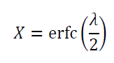
Using these axes, it can be seen that plotting measured data results in a situation where values can be interpreted as falling on a “universal curve” (figure 1).

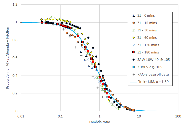
Figure 1 The variation of the proportion of mixed/boundary friction (X) with Lambda Ratio for a range of base oils [1] (Data is for surfaces with Gaussian height distributions and roughly equal roughness on each surface.)

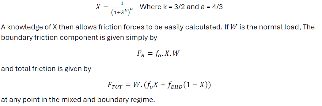
The fit curve to the data can be modelled by a simple reverse “S-curve” equation which relates the Lambda Ratio to the proportion of mixed/boundary friction “”, as follows:

The method described above also work well for lubricants that do not contain additives, and simple modifications can be made to account for friction modifiers and anti-wear additives in formulated oils [2]. For example, lubricants containing anti-wear additives (such as ZDDP) develop roughened surfaces due to the formation of the sacrificial anti-wear film during operation. Consequently, it is important to use the roughness values following a period of use. i.e., those which incorporate the anti-wear film characteristics, when calculating the Lambda Ratio.

Similarly, when lubricants with friction modifiers are used the appropriate value of .is required for the fit. However, in the case of such lubricants, each lubricant formulation seems to require a unique curve fit as data for these oils does not collapse onto a single curve.

More recently the above work has been extended and alternative equations, which do not contain any fitting parameters, yet provide good fits to experimental data, have been found. For example, for surfaces with Gaussian height distributions:

The main purpose of this newer work is to develop equations to predict mixed/boundary friction for surfaces which have different surface roughness height distributions, particularly to account the effect of changes in surface topography during running-in. [3]. While the above approaches offer a new and simple approaches to calculating mixed and boundary friction, this is not the first time that researchers have proposed simple equations relating X to lambda. Other similar equations have been proposed [4,5,6], but they have never been widely adopted, perhaps due (in some cases) to the fact that they are only applicable over limited ranges of lambda.

Is the back of an envelope all we need?

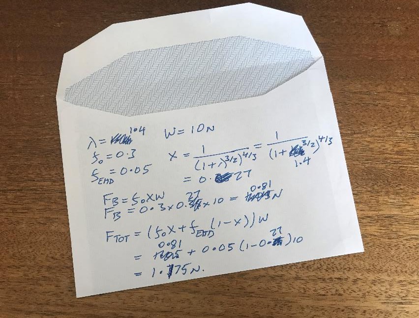
Research by Taylor and Sherrington is continuing, their hope is that these simple approaches become more widely applied as “back of an envelope” calculations (figure 2) or as simple spreadsheet calculations. They dispense with the need for complex models and detailed expert understanding and they can also easily amended with different values for sensitivity checks.

Increased use of this form of calculation may potentially expose “hidden” power losses. Of course, if tribologists can expose these places, it allows action to be taken to reduce their effect. In a broad sense this can lead to a reduction in the unnecessary use of energy, lowered economic losses, decreases in climate effects due to avoidable CO2 emissions and diminished use of raw materials, which are the goals of all engineers, economists and environmentalists.

References

Taylor, R. I. and Sherrington, I. “A Simplified Approach to the Prediction of Mixed and Boundary Friction”, Trib Int 2022;175;107836 https://doi.org/10.1016/j.triboint.2022.107836
Taylor, R. I. Sherrington, I. “Prediction of Friction Coefficients in Mixed Lubrication Regime for Lubricants Containing Anti-Wear and Friction Modifier Additives”. Tribology On-Line. 18 (4) (2023) pp 185 – 195. DOI https://doi.org/10.2474/trol.18.185
R. I. Taylor and I. Sherrington, “Modelling Mixed/Boundary Friction using the Lambda ratio and Overlap Coefficients for Realistic Rough Surface Height Distributions”. https://doi.org/10.1080/10402004.2025.2574843
A.V. Olver and H.A. Spikes, “Prediction of Traction in Elastohydrodynamic Lubrication”, Proc IMechE Part J, 212, 321- 332, 1998 https://doi.org/10.1243%2F1350650981542137
Castro, J., and Seabra, J. “Coefficient of Friction in Mixed Film Lubrication: Gears versus Twin-Discs”, Proc. IMechE.Pt. J: Journal of Engineering Tribology, 221, pp 399–411, 2007 https://doi.org/10.1243%2F13506501JET257
Zhu, D., and Hu, Y. A computer program package for the prediction of EHL and mixed lubrication characteristics, friction, subsurface stresses and flash temperatures, based on measured 3-D surface roughness. Trib. Trans. 44(3)(2001), pp.383-390 https://doi.org/10.1080/10402000108982471