







AI-Guided TriboSolver Workflow: Generated Surfaces, Analytical Checks, and Mesh Refinement
By Aydar Akchurin
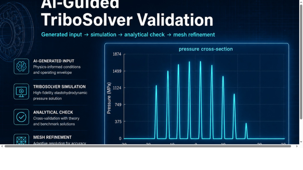
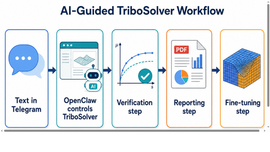
AI-guided TriboSolver experiment was setup to see the exten to which OpenClaw AI agent can control and run the simulations using TriboSolver. In this experiment a Telegram-controlled OpenClaw AI agent generated the input surface, operated TriboSolver through the web interface, extracted the result field, checked the result against an analytical Hertzian model, generated a report, and then refined the simulation when the first mesh looked suspicious. This represents the typical engineering simulation cycle.
Key takeaways:
- AI agents boost the usability of tools like TriboSolver by offering quick support in preparation, verification & post processing: creating surfaces, generating analytical solutions and creating customized reports can be done by the agent
- AI agents can control TriboSolver web tool robustly and turn a human-language instructions into a specific solver input/outptut, even without documentation and API
- Typical engineering simulation workflow can be set up and run on the background while the engineer can be doing other work
What we wanted to test
The goal was to run a controlled dry contact calculation where the input micro-geometry was created by the AI agent rather than selected from an existing file. The initial surface was a sinusoidal height field:
- Amplitude: ±50 nm
- Final wavelength / period: 4 µm
- Domain: 60 µm × 60 µm
- Surface import: one generated CSV surface applied in TriboSolver
Simulation setup in TriboSolver
The calculation was run as a dry contact simulation in TriboSolver using the Boundary Element Method. OpenClaw used the TriboSolver web workflow, uploaded the generated surface, started the calculation, loaded the result file, selected the result variables, and extracted the plotted pressure data from the Results tab.
- Simulation: Dry Contact Simulation
- Contact model: Boundary Element Method
- Friction model: none
- Normal load: 0.1 N
- Macro geometry: point contact
- Body radii: Rx = Ry = 1e-2 m for both bodies
- Body 1 material: E = 200 GPa, ν = 0.30, H = 2.0 GPa
- Body 2 material: E = 160 GPa, ν = 0.27, H = 9.5 GPa
- Final numerical grid: 256 × 256 × 32 over 60 µm × 60 µm × 60 µm
- Final lateral step size: 2.34375e-7 m
Generated solver input: from Telegram request to CSV surface
The important new feature in this workflow was that the input surface was generated as part of the run. Instead of offline preparing a micro-geometry file, the AI agent created a sinusoidal CSV matrix with the requested amplitude and wavelength, uploaded it through the TriboSolver interface, and entered the matching lateral step size.
This matters because a useful engineering workflow often includes:
- constructing or modifying a surface input,
- checking whether the mesh resolves the surface features,
- running the solver,
- extracting the output field,
- validating the scale of the result,
- and iterating when the result does not look physically or numerically convincing.
That complete loop is what was demonstrated here.
Analytical validation: Hertzian contact as the baseline
Before trusting the rough-surface pressure map, we checked the result against the corresponding smooth Hertzian point-contact solution. For the two elastic bodies used here, the effective modulus and radius are:
- Effective elastic modulus: about 96.7 GPa
- Effective radius: 5 mm
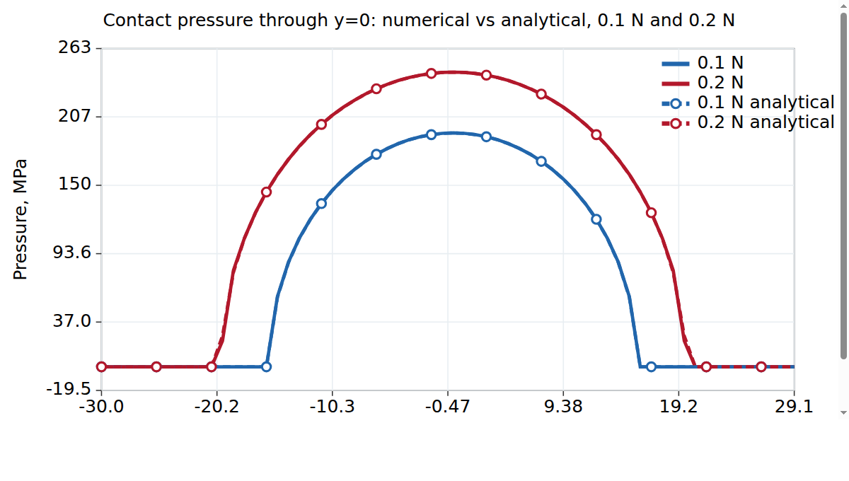
For a 0.1 N smooth Hertzian contact, this gives approximately:
- Hertz contact radius: 15.7 µm
- Hertz contact area: 7.76e-10 m²
- Mean Hertz pressure: 128.9 MPa
- Maximum Hertz pressure: 193.4 MPa
- Hertz indentation: 49.4 nm
The TriboSolver rough-surface result is not expected to match these pressures directly, because the sinusoidal topography concentrates the load on a much smaller real contact area. But the analytical model gives a sanity check for the load, geometry, indentation scale, and the smooth-contact reference pressure.
Final 256 × 256 TriboSolver result
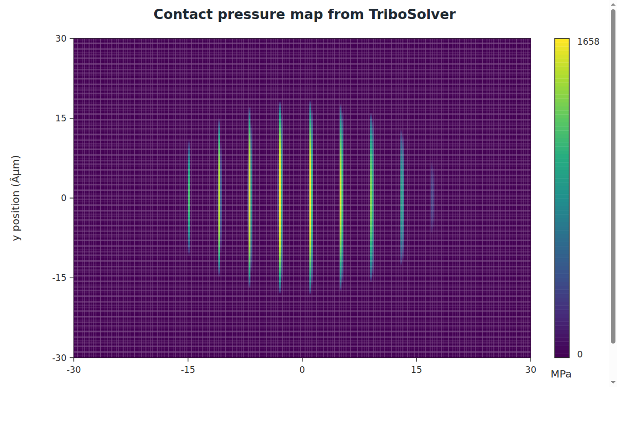
After refining the mesh to 256 × 256, the verified TriboSolver Results-tab metrics were:

| Metric | Final 256 × 256 result | Comment |
|---|---|---|
| Calculated contact load | 0.10000000000000007 N | Matches the requested 0.1 N load |
| Average contact pressure | 793.91 MPa | Higher than smooth Hertz because contact localizes on sinusoidal summits |
| Nominal contact pressure | 27.78 MPa | Based on the nominal simulation area |
| Rigid body motion | 54.37 nm | Same order as the smooth Hertz indentation |
| Real contact area | 1.2596e-10 m² | Much smaller than the smooth Hertz area |
| Peak contact pressure | 1658.01 MPa | Peak extracted from the PADIS pressure field |
The refined result is physically more plausible than the initial lower-density visualization because the 4 µm sine wave is represented by more points per wavelength. At 128 × 128, the lateral step was 0.46875 µm, giving only about 8.5 points per 4 µm wave. At 256 × 256, the step became 0.234375 µm, giving about 17 points per wave. That is still not infinite resolution, obviously, but it is a much better representation of the imposed sinusoidal geometry.
Why the first result looked wrong
The first 4 µm-period simulation at 128 × 128 did run successfully. However, the pressure plot looked too coarse for the intended interpretation. The numbers also shifted after refinement:
| Quantity | 128 × 128 | 256 × 256 |
|---|---|---|
| Lateral step size | 0.46875 µm | 0.234375 µm |
| Points per 4 µm wavelength | ~8.5 | ~17.1 |
| Average contact pressure | 641.0 MPa | 793.9 MPa |
| Real contact area | 1.56e-10 m² | 1.26e-10 m² |
| Peak contact pressure | 1426.8 MPa | 1658.0 MPa |
The agent can automate the rerun, but the decision to question the result still comes from engineering judgement. In this case, the visual pressure field and the mesh-to-wavelength ratio both suggested that the first mesh was not dense enough. Actually, that step probably also can be checked by the agent.
After the refined simulation, the agent generated a PDF report from the TriboSolver Results-tab data. The report included the generated surface profile, contact pressure map, and pressure cross-sections.
Additional use case: fractal roughness with Sq 10 nm and H = 0.8
As a second use case, the same OpenClaw-controlled TriboSolver workflow was used to generate and calculate the contact pressure for a random fractal roughness profile instead of the sinusoidal surface. The surface was generated by the agent and used a target root-mean-square roughness Sq = 10 nm, Hurst exponent H = 0.8, a 256 × 256 grid over the same 60 µm × 60 µm domain, and a measured generated-height range from about −27.16 nm to +31.04 nm. This surface was imported into TriboSolver as the micro-geometry input and run with the same dry-contact BEM setup at 0.1 N. The verified Results-tab values were: calculated load 0.10000000000000003 N, average contact pressure 266.11 MPa, nominal pressure 27.78 MPa, rigid body motion 60.28 nm, real contact area 3.7579e-10 m², and peak contact pressure 2000 MPa. The key point is that the agent did not only repeat one predefined surface: it generated a statistically defined rough surface, passed it to TriboSolver, extracted the solver result, and produced a report from the UI result data.
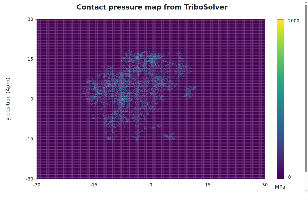
Download the fractal roughness Sq 10 nm / H = 0.8 dry contact PDF report
What this says about AI in tribology simulation
The useful role of AI here was as follows:
- turning a short Telegram instruction into a specific solver input,
- operating the TriboSolver interface consistently,
- extracting result fields for custom plotting,
- checking the result scale against an analytical model,
- creating a report,
- and refining the mesh after the result was questioned.
That is a practical direction for engineering software. AI agents can help with setup generation, repetitive UI work, comparison, reporting, and iteration. The engineer owns the model assumptions and the final judgement.

Key takeaways:
- AI agents boosts the usability of tools like TriboSolver by offering quick support in preparation, verification & post processing: creating surfaces, generating analytical solutions and creating customized reports can be done by the agent
- AI agents can control TriboSolver web tool robustly and turn a human-language instructions into a specific solver input/outptut, even without documentation and API
- Typical engineering simulation workflow can be set up and run on the background while the engineer can be doing other work
0 Comment