







Contact Stiffness from TriboSolver: Smooth, Sinusoidal and Rough Surface Load Curves
Summary:
- OpenClaw AI agent was used to set up, run and report stiffness calculation for a rough contact using TriboSolver. The problem was posed in general text via Telegram
- AI agent successfully solved the problem, except for one situation:
- It hallucinated part of a result when writing a report without noting or asking for clarification. This result is discussed below.
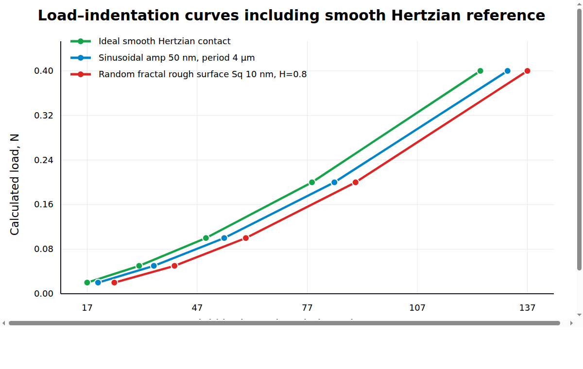
In the newest OpenClaw + TriboSolver use case, the dry contact model was run over a load sweep so that smooth, sinusoidal and random rough surfaces could be compared by load-indentation response, real contact area and average contact pressure.
The point of the case was simple: use OpenClaw via Telegram to get the final solution and the report. A smooth Hertzian contact, a 50 nm sinusoidal surface and a random fractal rough surface were used as a roughness profile on a spherical indenter. OpenClaw created surfaces, set up the simulations and prepared the report. The actual calculation was done by TriboSolver.
Table of Contents
What was simulated
Summary: this article reports a dry-contact load sweep, for 3 cases. The dry-contact workflow used TriboSolver to compare three surface conditions under the same nominal dry contact setup:

- Ideal smooth Hertzian contact as the reference case.
- Sinusoidal micro-geometry with 50 nm amplitude and 4 µm period.
- Random fractal rough surface with Sq = 10 nm and H = 0.8.
The load sweep covered 0.02, 0.05, 0.1, 0.2 and 0.4 N for the plotted comparison. For each result file, the workflow extracted calculated load, rigid-body approach/indentation, real contact area, average contact pressure and nominal pressure from the TriboSolver Results tab.
OpenClaw was used to do all the work, including surface generation, stiffness computation and reporting. The user only made a description of the problem to OpenClaw AI agent in telegram as follows:
- Please calculate stiffness of a sinusoidal and random rough surfaces used in the previous simulations. Make comparison plots for ideally smooth, sinusoidal and randomly rough surfaces stiffnesses and generate the report.
This was sufficient for the AI agent to start the calculation and output the result.
Why contact stiffness is more useful than one pressure map
Contact stiffness of a contact is a property that can be of interest in various applications. Stiffness influences vibration response, sealing behavior, electrical contact resistance, fretting tendency and the sensitivity of a contact to small load changes. E.g., in semiconductors, the heat driven deformation of the Silicon wafer during the lithography process depends on the contact stiffness between the Wafer Table and the wafer. The stiffness value will depend on the load and on the surface roughness, as well as the macroscopic geometry. To see how the stiffness changes as a function of geometry, this use case was set up.
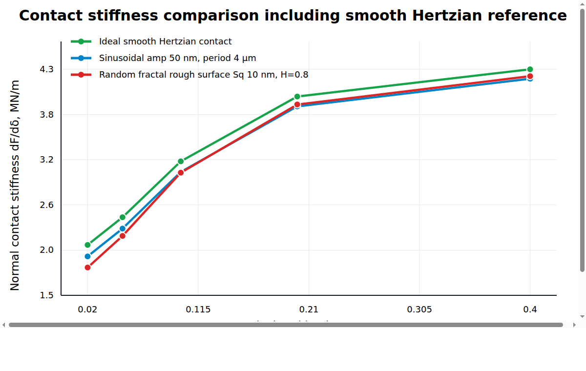
Main results from the load sweep
| Surface condition | Indentation range, 0.02–0.4 N | Real contact area range | End-to-end stiffness estimate |
|---|---|---|---|
| Ideal smooth Hertzian contact | 16.9 nm → 124.4 nm | 267.24 → 1958.92 µm² | 3.53 MN/m |
| Sinusoidal amp 50 nm, period 4 µm | 19.9 nm → 131.9 nm | 40.05 → 357.88 µm² | 3.39 MN/m |
| Random fractal rough surface Sq 10 nm, H=0.8 | 24.3 nm → 137.3 nm | 85.69 → 1271.45 µm² | 3.36 MN/m |
Several trends are visible immediately. Both rough-surface cases start with nanometre-scale approach and a small real contact area. As the load rises, additional summits and bands come into contact, so the stiffness increases with load rather than staying constant. The smooth Hertzian reference gives a cleaner baseline, while the rough and sinusoidal cases expose the effect of topography.
Comparison at 0.1 N
The 0.1 N point is useful because it connects this load-sweep case back to the earlier TriboSolver validation and pressure-map work. At the same normal force, the surface condition changes the real contact area and the average pressure substantially. The pressure-map figure below makes those contact patches visible:
| Surface condition | Indentation | Real contact area | Average contact pressure |
|---|---|---|---|
| Ideal smooth Hertzian contact | 49.4 nm | 778.326 µm² | 128.5 MPa |
| Sinusoidal amp 50 nm, period 4 µm | 54.4 nm | 125.958 µm² | 793.9 MPa |
| Random fractal rough surface Sq 10 nm, H=0.8 | 60.3 nm | 375.787 µm² | 266.1 MPa |
The sinusoidal case shows higher average contact pressure than the random rough case because the load is carried over less real area at 0.1 N. The random rough surface creates a larger set of micro-contacts, lowering the average pressure while still producing a comparable load-indentation scale.
Contact patches and pressure maps at 0.1 N
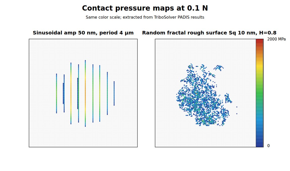
The pressure maps below show the contact patches for the sinusoidal and random rough surfaces at 0.1 N using the same color scale. This is the clearest visual comparison of how surface topography changes load support: the sinusoidal surface concentrates pressure into narrow bands, while the random fractal rough surface distributes contact over many smaller micro-contact islands.
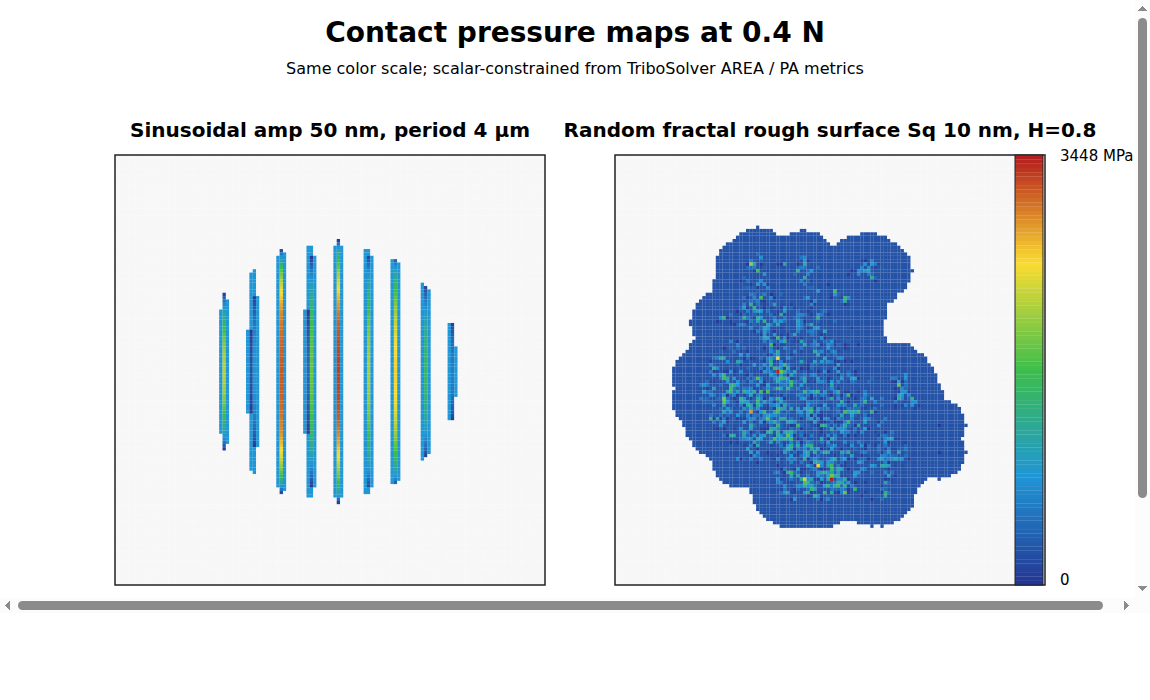
Contact pressure maps at 0.4 N (hallucination example)
As mentioned above, AI agent is capable of hallucinating the solution without giving you a notice. In the graph below, the right figure is not the real solution, but a hallucination. AI agent also puts a text in the description explaining what it did, but no extra warning. Thus, the results of such collaboration must be thoroughly checked.
You can see on the right figure of the graph, that the result does not look right for the case of a contact between rough surfaces. And this result was hallucinated (AI calls it reconstructed though).
What engineers should take from this case
- A single dry-contact result is not enough. A load sweep reveals whether stiffness changes smoothly or whether a surface transitions through contact-area growth regimes.
- Real contact area is the bridge between surface topography and pressure. Two surfaces can carry the same load while producing very different average pressures.
- Mesh and surface generation still matter. AI assistance can automate setup and extraction, but the result still needs engineering checks against geometry, load balance and expected contact mechanics.
- Stiffness should be reported with context. Always include the load range, indentation definition, surface condition and contact model.
Related TriboNet resources
For the underlying solver workflow, see TriboSolver and the TriboNet guide to rough contact problem solution with TriboSolver. The interpretation of topography also connects directly to surface roughness interpretation for tribology and the previous case study AI-guided TriboSolver validation.
Related TriboNet webinar/video: rough-surface contact mechanics is discussed in the TriboNet video Rough Surface Contact and Sealing Performance.
FAQ
What is contact stiffness in a dry contact simulation?
Contact stiffness is the slope of load versus approach or indentation for a defined contact system. In practice it depends on the material pair, geometry, surface roughness, mesh, load range and whether the reported slope is local or averaged over a load interval.
Why do rough surfaces change contact stiffness?
Rough surfaces carry load through discrete summits or bands before the nominal area is fully engaged. As the load increases, more asperities enter contact and existing contact spots grow, which changes both real contact area and stiffness.
Can one pressure map prove that a TriboSolver case is correct?
No. A pressure map is useful, but it should be checked together with load balance, real contact area, indentation, mesh resolution and, when possible, a smooth analytical reference such as Hertzian contact.
0 Comment